Graph outlining the Change Vector Analysis – updated version based on the graph from Chapter 9.
We explained in Chapter 9 among other change detection methods also the change vector analysis practically using the rasterCVA() command in the RStoolbox package, as well as outlined the approach graphically. During my last lecture on temporal and spatial remote sensing approaches I realized that the graphic needs some fixing as well as the RStoolbox function, moreover, certain explanations were missing. Hence, Benjamin Leutner adapted the rasterCVA() command and I tested it again and created new graphics explaining this approach for land cover change analysis.
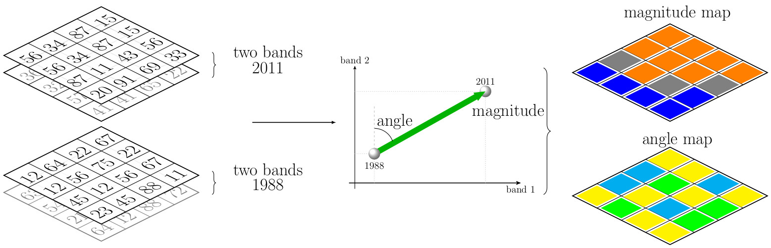
The first (slightly modified) graph that is also in our book shows the general approach. Two bands for each year (e.g. the RED and NIR band) are taken and the changes in pixel values between these two years are shown as angle and magnitude.
We realized some things were missing:
- the explanation what the angle actually means
- a link of actual results and the xy-graph.
- and an example using e.g. Tasseled Cap
In the following new figures we show the actual results of the land cover change vector analysis using band 3 and 4 of Landsat (E)TM for the study region used in our book and three angles and magnitudes of pixels values between 1988 and 2011.
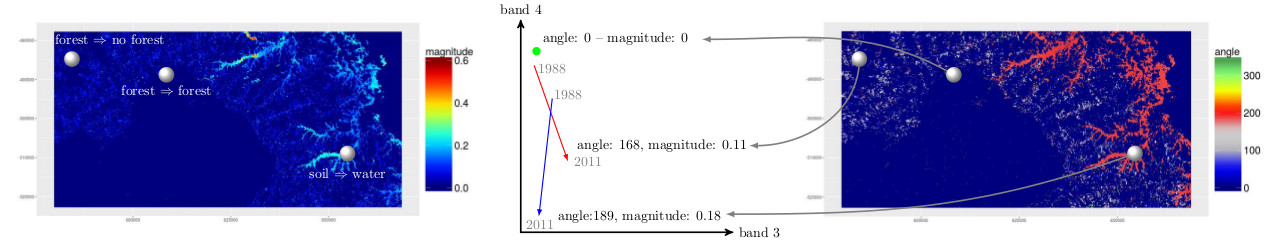
Change Vector analysis explained on three change classes using the actual rasterCVA() output and band values.
In the second image we outline the meaning of the angle provided by rasterCVA() as well as the magnitude which is the euclidean distance of the pixel values between time-step 1 and time-step 2. The actual bands are shown on the x-axis (first band assigned in the command) and y-axis (second band):
Meaning of the angle values from a rasterCVA() output.
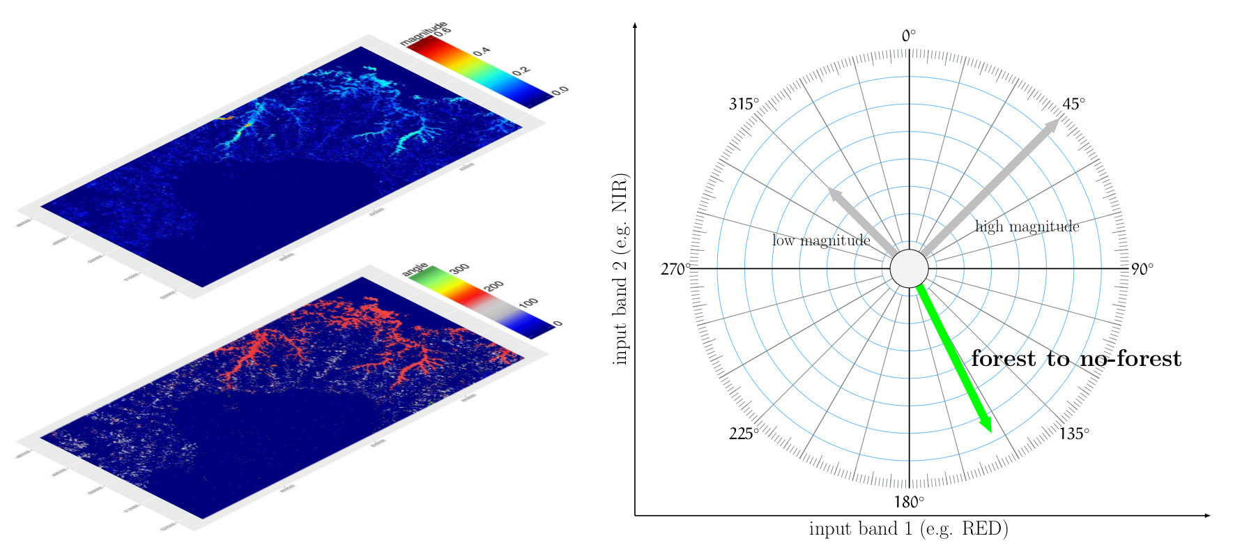
In another graph we just show the angle and magnitude of a forest to no-forest conversion between time-step 1 and time-step 2. This one if very similar to the above graph but we just assigned the start and end location of the change vector to actual band 3 and band 4 values:
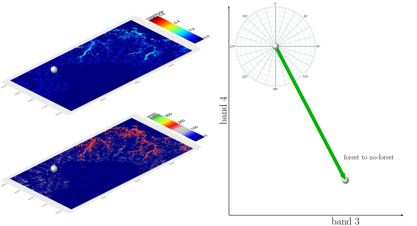
Actual angle and magnitude using band 3 and band 4 for a forest to no-forest conversion pixel.
Similar results can be achieved using the Tasseled Cap output (greeness and wetness, from tasseledCap() command) as input for the change vector analysis. The map looks similar (we used as input the masked Landsat data in order to avoid the high magnitude values in the inundated areas for visualization purpose), but the actual change vector angle for the forest to no-forest conversion is different:
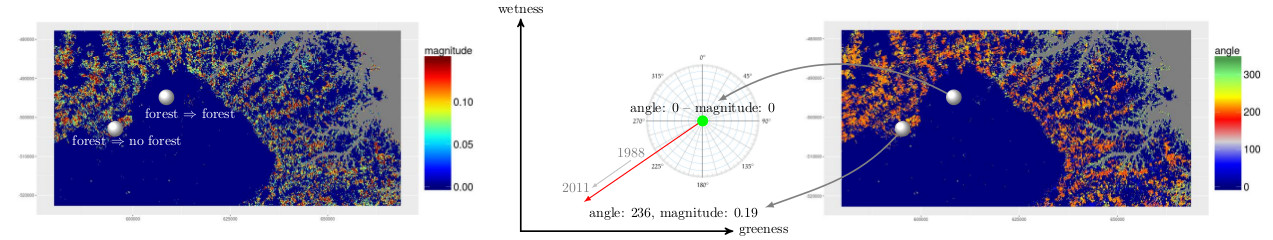
Change Vector Analysis results using wetness and greenness for two locations of forest to forest and forest to no-forest conversion.
Please update to the newest development version to access the updated RStoolbox functionality to redo these analysis. Please contact us for any recommendations concerning these graphs.